Expected Goals: What xG Actually Measures
Published 1/20/2026 · 13 min read · Sport calculators

Expected goals is the probability that a shot with a given set of features becomes a goal, estimated by fitting a model to a very large sample of historical shots. Opta trains on nearly a million of them and weighs more than twenty variables per shot — distance, angle, body part, the pattern of play that produced the chance, the goalkeeper's position, the bodies in the way. The output is a number between 0 and 1, and it is a model output, not something anyone observed: the shot either went in or it did not. Sum the shot probabilities and you get a team's xG for a match. That sum behaves very differently from the scoreline. Take a team that fires 22 shots from distance, 18 of them worth 0.03 and 4 worth 0.05: total xG 0.74, and a 47.1% chance of not scoring at all. Against it, a team with 7 shots including a penalty at Opta's fixed 0.79 totals 1.53 — more than double, on a third of the volume. Strip the penalty and its remaining six shots come to exactly 0.74, the same as the other side's 22. That is what xG measures: chance quality, not chance quantity.
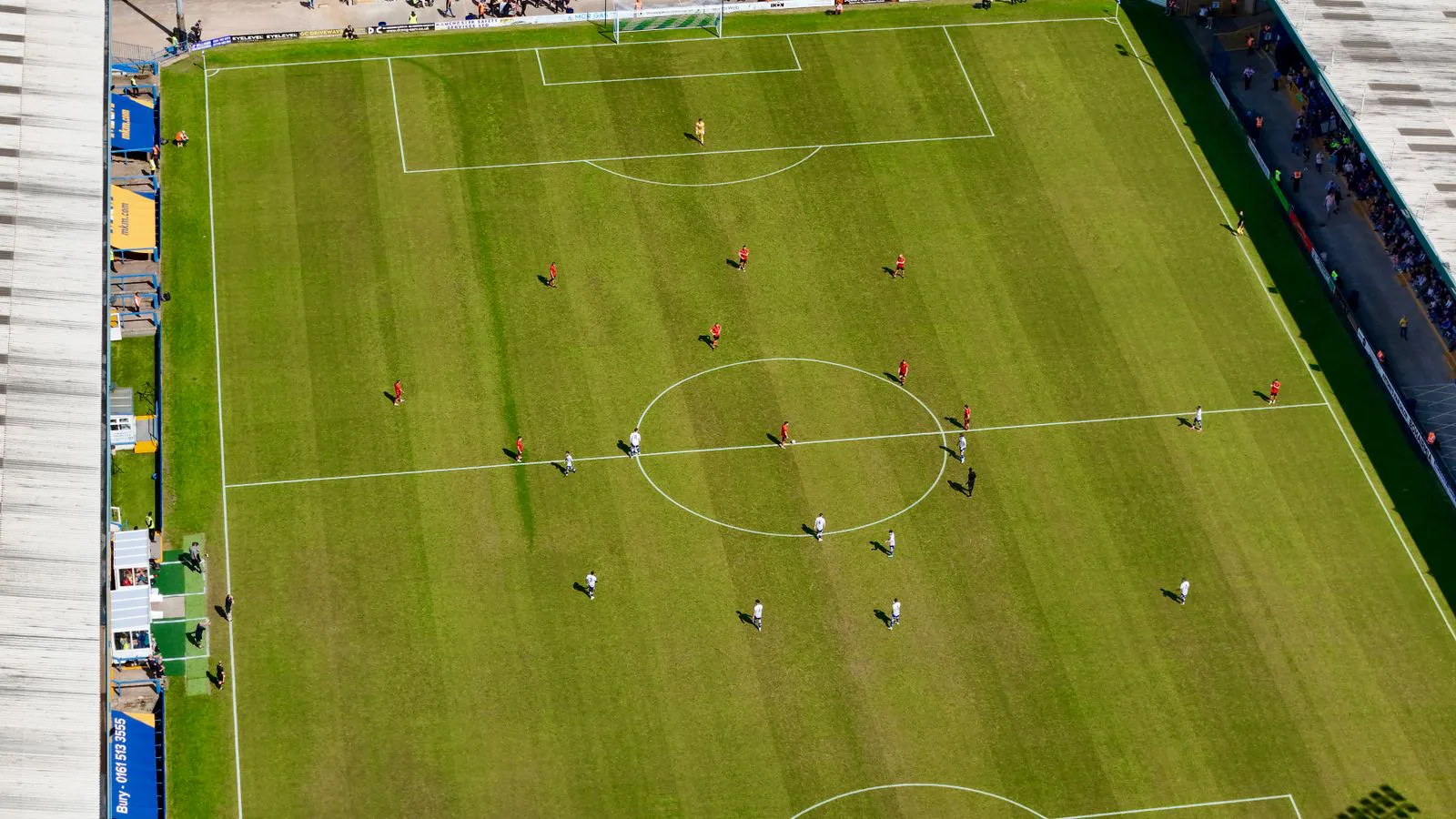
xG is the fitted probability that a shot with a given set of features becomes a goal — a model output, not an observation. A worked match, the binomial arithmetic that says one game is far too few shots, and the limits nobody quotes.
A probability, fitted — not a measurement, taken
An xG model is a classifier. It is handed a large archive of shots, each labelled goal or no goal and described by a list of features, and it learns a function that maps those features to a probability. Opta's public description names the ingredients: distance to goal, angle to goal, the body part used, whether it was a volley or a header or a one-on-one, the pattern of play that created the chance, the previous action, the goalkeeper's position, how much of the goalmouth was visible, and the pressure from defenders — more than twenty variables in all, fitted on close to a million historical shots.
The consequence is easy to state and constantly forgotten. A shot valued at 0.33 did not produce a third of a goal. It produced either one goal or none, and 0.33 is the model's estimate of how often shots resembling it have gone in. The number describes a reference class, not the event. That is why an xG figure has no error bar attached in most public displays but deserves one, and why two providers looking at the same shot can and do return different numbers — they are describing different reference classes, because they measured different features.
The match where the shot count lies
Team A has the ball, camps in the opposition half and shoots 22 times, almost always from outside the box against a set defence. Give 18 of those shots a model value of 0.03 and the four best of them 0.05. The match total is 0.74, and the average shot is worth 0.034. Team B defends, breaks three times and wins a penalty. Its seven shots are one penalty at Opta's fixed 0.79, a clear chance at 0.33, a half-chance at 0.21 and four hopeful efforts at 0.05. The match total is 1.53, and the average shot is worth 0.219 — six and a half times Team A's.
Two arithmetic facts make the point better than any adjective. First, the penalty on its own is worth 0.79, which is more than Team A's entire evening of 0.74 — one kick against 22 attempts. Second, if you delete the penalty from Team B's card, its remaining six shots add up to exactly 0.74, the same total Team A needed 22 shots to reach. The count of shots and the quality of shots are two different measurements, and only one of them is about scoring. It takes 26.3 shots at 0.03 to accumulate the expectation of a single penalty.
One big chance against many small ones
Because the shots are independent under the model, you can turn the two lists into full distributions rather than single totals. Team A's 22 low-value shots give a 47.1% chance of scoring none, 36.1% of scoring once, 13.2% of scoring twice. Team B's seven shots give only a 9.1% chance of a blank, 42.8% of one goal and 35.8% of two. The gap in the probability of at least one goal is enormous — 52.9% for A against 90.9% for B — and it comes almost entirely from the penalty, which alone carries a 79% chance of a goal against A's 22 shots collectively carrying 52.9%.
Convolve the two distributions and you get the model's view of the result: Team B wins 61.9% of the time, the match is drawn 24.8% of the time, and Team A — with three times the shots and half the chance quality — still wins 13.3% of the time. That last figure is the honest caveat on every xG post-match graphic. Doubling your opponent's xG in a single match leaves you failing to win it in more than a third of simulated evenings. xG does not say who deserved to win. It says what the chances were worth, and the chances were worth a result that arrives only most of the time.
Why xG predicts goals better than goals do
The finding that xG totals forecast future goals better than past goals do has been replicated repeatedly, and the reason is not mystical. Goals are a low-count outcome drawn from a high-variance process. If a team takes 13 shots a match and each is worth 0.10, its expected haul is 1.30 goals with a standard deviation of the square root of 13 x 0.10 x 0.90, which is 1.08 — a spread of 83.2% of the mean. Over a season of 494 shots the expectation is 49.4 goals with a standard deviation of 6.67, and a 95% band running from 36.3 to 62.5. Even across a whole season, chance moves the goal column by a quarter of its own size.
The xG sum, by contrast, carries none of that Bernoulli noise. It is a deterministic function of the shots taken: the same shots always produce the same total, whatever the goalkeeper happened to do. So goals equal xG plus noise, and forecasting next season from this season's goals means forecasting from the signal and the noise together, while forecasting from xG uses the signal alone. That is the whole mechanism. It also tells you when the argument stops working: if a team's shots really are being taken by a finisher who beats the model, or against a goalkeeper who beats it, the difference is signal too, and xG is throwing it away. Distinguishing the two takes hundreds of shots.
How many? Set a target for the relative standard deviation of the goal count and solve. With a shot worth p, you need n at least (1 − p) / (p t²) shots to get the relative standard deviation down to t. At p = 0.10, reaching 20% takes 225 shots, about 17 matches. Reaching 10% takes 900 shots, about 69 matches — nearly two seasons. Reaching 5% takes 3,600. A single match of 13 shots sits at 83.2%, which is another way of saying that a one-match xG figure is a headline and not a measurement.
The same shot, two models, two numbers
Start with the easiest shot in football to model. A penalty is taken from a fixed spot, with a fixed distance and angle, against one goalkeeper, with nobody else allowed inside the box. Every provider treats it as a constant rather than running it through the model. Opta's constant is 0.79. Statsbomb's, after its 2022 update, is 0.78. The most standardised event in the sport, with tens of thousands of historical instances, and the two best-known models still differ in the second decimal place. That is not an error by either of them — it is what happens when two teams choose two historical samples.
Away from the penalty spot the divergence is far larger, because it stops being about the sample and starts being about which features exist at all. Statsbomb's published illustration is exact: a model built on distance, angle, body part and assist type values a particular chance at 0.30, while a model that also knows where the goalkeeper was standing, where every attacker and defender in frame was, and how high the ball was at impact values the same chance at 0.65. More than double, for one shot, from adding information rather than changing method. When two sites report different xG for the same match, this is usually why — and it is why an xG figure without the name of the model attached is an incomplete quantity.
What the number does not know
Four limits deserve to be quoted every time the figure is. The first is defensive context: most freely available models see distance, angle and body part but not the defender arriving, so a shot taken under a sliding challenge and the same shot taken unmarked can carry the same value. The second is independence: the model adds shot probabilities as though each were a separate draw, but a rebound only exists because the first shot was saved, and a team that has just won a corner is more likely to shoot again in the next twenty seconds. Adding those probabilities overstates the spread of possible scorelines slightly, and understates how clustered chances really are.
The third is the penalty. Its fixed value is by a wide margin the largest single number on most match cards, and in the worked example above it is 51.6% of Team B's entire total — one refereeing decision accounting for more than half of a team's measured attacking output. Over a season that averages out; over one match it dominates, and it is worth reading any small-sample xG figure twice, once with penalties and once without. The fourth is game state: a team leading 2-0 with twenty minutes left stops attacking, and its xG falls for a reason that has nothing to do with how good it is. None of these makes xG a bad number. They make it a number with a stated scope, which is the only kind worth quoting.
| Line | Shots | How the total is built | Total xG | xG per shot | What the model says |
|---|---|---|---|---|---|
| Team A | 22 | 18 shots at 0.03 + 4 at 0.05 | 0.74 | 0.034 | 47.1% chance of not scoring at all |
| Team B | 7 | 0.79 penalty + 0.33 + 0.21 + 4 at 0.05 | 1.53 | 0.219 | 9.1% chance of not scoring at all |
| Team B, penalty removed | 6 | 0.33 + 0.21 + 4 at 0.05 | 0.74 | 0.123 | Identical to Team A's whole match, on six shots instead of 22 |
| The penalty alone | 1 | Opta's fixed value for a penalty | 0.79 | 0.790 | Worth more than Team A's entire 22 shots |
Frequently asked questions
- Is a 0.5 xG chance worth half a goal?
- No. It is the model's estimate that about half of the shots resembling that one, in its training data, ended up in the net. The particular shot produced one goal or none. Half a goal is a useful bookkeeping device when you add many chances together, because expectations add even when the individual outcomes are all-or-nothing, but it is never a description of what happened on the pitch. The moment you say a player missed half a goal you have swapped a probability for an observation.
- Why do two websites report different xG for the same match?
- Because they are running different models on different feature sets. A model that knows only distance, angle, body part and assist type sees a different shot from one that also knows the goalkeeper's position, every player in frame and the height of the ball at impact — Statsbomb's own published example has those two models valuing one chance at 0.30 and 0.65. Even on penalties, where every model uses a flat historical rate, Opta uses 0.79 and Statsbomb 0.78. Quote the provider alongside the number, and never compare an xG total from one source with an xG total from another.
- Should I strip penalties out of an xG total?
- For small samples, look at both. A penalty carries a fixed value near 0.79, which makes it several times larger than any other shot on the card; in the match worked through above it is 51.6% of one team's entire total. That is one refereeing decision determining more than half of a measured attacking performance. Over a full season penalties are a real and repeatable part of what a team generates, so leave them in. Over one match or five, the non-penalty figure tells you far more about how the team is creating chances.
- How often does the team with more xG actually lose?
- Often enough that the question should be asked before the graphic is posted. In the match worked through in this article, one team more than doubles the other's xG — 1.53 against 0.74 — and the model still gives it only a 61.9% chance of winning, with 24.8% for a draw and 13.3% for a defeat. So the better chances fail to bring three points on more than a third of simulated evenings. That is not xG being wrong. It is xG being a probability and being read as a verdict.
- Does xG tell me whether a striker is a good finisher?
- Not on the evidence of one season. The usual test is goals minus xG, and the arithmetic above says how noisy that difference is: at 13 shots a match and an average shot worth 0.10, the standard deviation of the goal count over a full season of 494 shots is 6.67 goals. A striker five goals above his xG has produced a gap smaller than one standard deviation of pure chance. Getting the relative noise down to 10% needs about 900 shots, which for most forwards is several seasons. The signal exists — some players really do beat the model — but you need years of data to see it.
Articles you may find interesting
All guides →Related tools
Sources
- Opta Analyst — What is Expected Goals (xG)?
- Hudl Statsbomb — What are Expected Goals (xG)?
- American Soccer Analysis — The Replication Project: Is xG The Best Predictor of Future Results?
- American Soccer Analysis — What are Expected Goals (xG)? — methodology explanation
- PLOS ONE — Expected goals in football: Improving model performance and demonstrating value
Spotted a mistake in this article?